The freeware OpenOffice spreadsheet application, which you add to your Windows XP, Vista, 7, 8, 8.1, Mac OS X or Linux software library from this website, is one with a variety of formatting options. Among them is a conditional formatting option, which applies certain formatting to cells based on a condition. For example, a condition could be if you input a number more than, less, than or equal to 10. Then that would trigger a change in the background color of the cell where you input the number.

To add conditional formatting to your spreadsheet, you must first set the formatting for a cell. Click on Format and Styles and Formatting to open the window in the shot below. It is there you can add new cell formatting based on a specific condition.

Click on the New Styles from Selection option, and then add a formatting such as Turn Red. That would be suitable if the formatting will turn the cell red. Then right-click Turn Red, or whatever you added, and select Modify to open the window below.

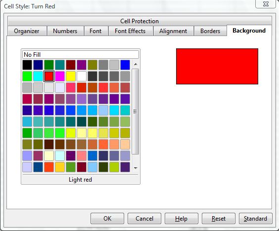
From that window you can set up all sorts of conditional cell formatting. To switch the cell color to red, click the Background tab and then a suitable color from the palette. Then click OK to save the formatting.

Click a cell, or select a group of cells on the spreadsheet, to add the conditional formatting to. Then click Format > Conditional Formatting to open the window below. It is there that you input the conditions for the formatting.

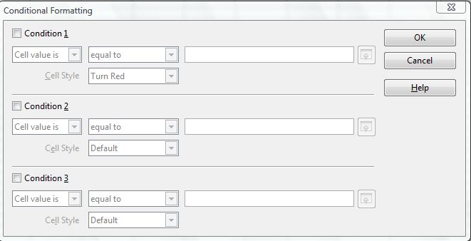
Click on the Condition 1 check-box, and select Cell value is from the drop-down list on the far left of the window. Choose a suitable condition from the adjacent drop-down list such as greater than. Then type in a value such as 10 in the text box. In the shot below, I have set a condition which will change the formatting of the cell when a number greater than 10 is put in the cells.

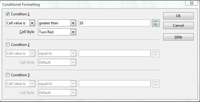
Then you should select some formatting for the cells from the Cell Style drop-down list. Choose the new formatting that you added, such as Turn Red, and then click OK. Return to the spreadsheet, and input a value into the cell that will alter the formatting based on the condition that you added. In the spreadsheet below, the selected cells turn red when I input a value higher than 10 in them.

Conditional formatting options add considerable flexibility to spreadsheets. With conditional formatting you can add variable formatting to a spreadsheet based on its cell content to highlight if specific values are reached, fallen below, equaled etc. Software such as Excel also have comparable options.