If you have an Excel spreadsheet with lots of data it might take a while to manually check through it for duplicated values. One way that you can quickly find duplicated cell values is with the Conditional Formatting option. When selected, the conditional formatting highlights any cells that include duplicated numerical values.

To add the conditional formatting to the whole spreadsheet, select the small box above row 1 and to the left of column A. That selects all the spreadsheet cells as in the shot below. Alternatively, select a smaller group of cells by left-clicking and dragging the mouse over them.

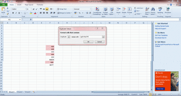
Once you have selected some cells, click on the Conditional Formatting option. Then click Highlight Cell Rules and Duplicate Values. That opens the Duplicate Values window below where you can choose the conditional formatting for the cells.

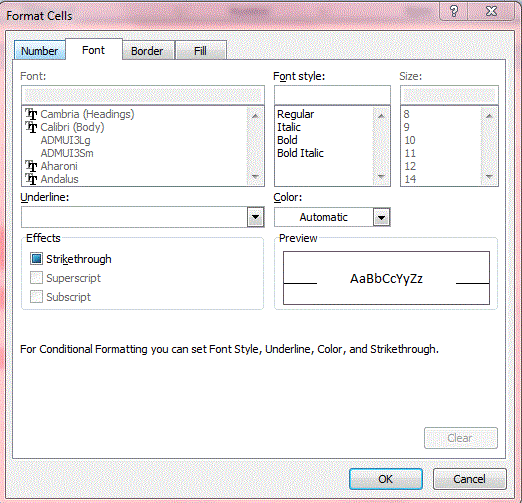
There you should select Duplicate and one of the formatting options such as Light Red Fill with Dark Red Text. Or you could select Unique cells instead which will add formatting to all those cells that do not have duplicated numbers. Click Custom Format to open the Format Cells window below where you can select further conditional formatting options.

Then click OK to close the window, and some of the formatting of the selected cells might switch to alternative colors as in the shot below. If you selected Duplicate from the Duplicate Values window, the conditionally formatted cells have duplicated values in them. Remove the duplicate values to erase the formatting.

The Duplicate Values option is just one of the great Excel conditional formatting options. With it you can find and edit all the duplicated data in your spreadsheets more effectively.