Email article
The “Find and Replace” function or Ctrl + F is a nice feature in MS Office, and we all know how useful it is; however, it does not seem to work in an Excel spreadsheet having thousands of cells as it gives you the following error message:
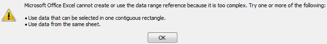
So, how to locate and highlight cells having a certain keyword in excel that has thousands of cells? There seems to be a workaround!
Highlight cells having keywords in an Excel spreadsheet with thousands of cells
Go to any cell having the keyword you are looking for, say, violet (not case sensitive). Or, let the cursor be present in any of the cells (it doesn’t matter). In Home tab, click Conditional Formatting, and then click Manage Rules. It will open a new window, “Conditional Formatting Rules Manager”. Click New Rule to open a new window, “New Formatting Rule”. Select Use a formula to determine which cells to format. Type in the following formula in the box below ‘Format values where this formula is true’:
=ISNUMBER(SEARCH(“VIOLET”,D1))
where D1 is the cell where you see your keyword ‘violet’.
Click Format to open a new window “Format Cells”. Go to the Fill tab, select any color you like (this will become the color of the cells having your keyword; so, try choosing a color that is more likely to draw your attention). You could choose some other formatting tab like Number, Font, or Border; but, highlighting a cell by a color is known to be most effective. Click OK. Click OK again. You can see your conditional formatting in the “Conditional Formatting Rules Manager” window. Go to the box of ‘Applies to’, and type =$D$1:$D$100000 instead of =$D$1 (that you see) if your data ends at the row of D100000. Check the box ‘Stop If True’.
All the cells having the keyword ‘violet’ should now be highlighted with the color of your choice. Don’t seem to be working? No worries, it’s not you, it’s Excel that might have changed the formula! What a shame! Fortunately, it won’t do it again if you go back to the “Conditional Formatting Rules Manager” window, and fix it. What a relief! To make sure that the rule you created is visible, select This Worksheet instead of Current Selection from the drop-down menu of ‘Show formatting rules for’ in the “Conditional Formatting Rules Manager” window. Now, click the ‘Rule’ to select it. Click Edit Rule. This will open the “Edit Formatting Rule” window. Change the formula as desired, and click OK.
Tip: NEVER try editing the formula here as Excel may not allow you to do it as smoothly as you want. For example, you could not use arrows on the keyboard to navigate as Excel would mess around with the formula. Therefore, use the copy & paste method, i.e., copy the formula from the other location, and paste it here. Now, check whether the formula in the box of ‘Applies to’ looks fine; if fine, click OK. You are good to go this time.
You may need to create multiple rules with multiple keywords (just choose different colors for different rules). For example, for some ‘mutually exclusive’ names like violet, indigo, blue, green, yellow, orange, red and so on. Alternatively, just create a single rule having all the keywords you want to look for!!! For instance, the following formula could be used to highlight all the cells having the keywords ‘violet, indigo, blue, green, yellow, orange, red’:
=OR(ISNUMBER(SEARCH(“VIOLET”,D1)),ISNUMBER(SEARCH(“INDIGO”,D1)),ISNUMBER(SEARCH(“BLUE”,D1)),ISNUMBER(SEARCH(“GREEN”,D1)),ISNUMBER(SEARCH(“YELLOW”,D1)),ISNUMBER(SEARCH(“ORANGE”,D1)),ISNUMBER(SEARCH(“RED”,D1)))
No need to worry about the uppercase or lowercase formatting as Excel doesn’t care, and will convert all of them to the uppercase format anyway.
Tip: There are possibilities of spelling mistakes in the database like ‘yelow’ instead of ‘yellow’ (imagine a humongous Excel spreadsheet having thousands of rows); so, to make the search more effective, use ‘yel’ as keyword!
I have tested this using Microsoft Office Excel 2013 in Windows 7 Professional 64 bit.
Did this tutorial excite you? Help you? Share it with your acquainted ones! Troubleshooting?
Let us know in the comments!