RANK.AVG and RANK.EQ are new Excel 2010 functions. They aren’t included in other versions except Excel 2013. These functions show you the statistical rank of a value within a list. So the rank tells you their order in a list of values.

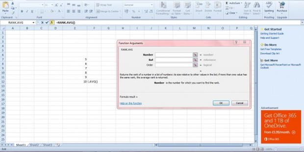
For example, enter 5, 6, 7, 8, 9 and 10 in an Excel spreadsheet column. Select a cell to add the RANK.AVG function to, and click the fx option. Then select RANK.AVG to open the window below.

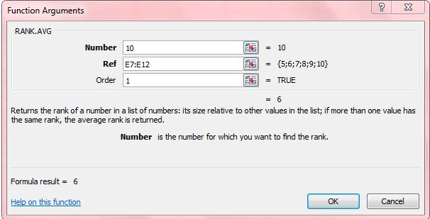
Enter 10 in the Number text box. Press the button beside the Ref field, and select the six cells you entered the numbers in.  Next, enter 1 in the Order field, which will rank 10 in ascending order.

Press OK to close the window. The function cell will have a value of 6. That ranks 10 as the sixth highest number in the list. Had you entered 0 in the Order field, the rank would instead be descending; and the value in the cell would be 1.

You can also use the RANK.EQ function to rank values in lists. The difference is that RANK.EQ returns the lowest rank for duplicate values. RANK.AVG returns the average rank for duplicate values.

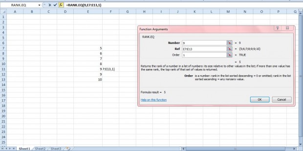
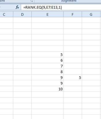
For example, enter an extra 9 in the column so that it includes 5, 6, 7, 8, 9, 9 and 10 as in the snapshot below. Then click a blank cell, press fx and select RANK.EQ from the Insert Function window. There enter 9 in the Number field, select all the cells in the list for the Ref field and input 1 in the Order text box.

Now click OK to add the function to spreadsheet. The RANK.EQ function cell will include 5 in it. As there are two nines in the list it ranks the lowest duplicate value. As such, nine is ranked fifth instead of sixth. The RANK.AVG function would have returned an average rank of 5.5 for the value in the same list.

So these functions enable you to rank values in Excel 2010/13 spreadsheets. Those with other versions of Excel can add RANK functions to spreadsheets. This YouTube video tells you about the RANK and RANK.AVG functions.