Those who have very large Excel spreadsheets can reduce them in size by removing a few rows or columns. Excel 2010/13 includes Hide/Unhide options with which you can temporarily remove columns and rows from view. As such, you don’t have to delete any rows or columns and then select the Undo option to put them back in the spreadsheet.

To hide a few rows from a spreadsheet, press the Ctrl key and select the rows to remove. Then right-click their row numbers on the far left of the spreadsheet, and select the Hide option. The selected rows should then disappear from the Excel spreadsheet.

To put them back, select the rows directly above and below the ones you removed from the spreadsheet. Then you should right-click the selected row numbers, and click the Unhide option. The rows should then reappear in the Excel spreadsheet.

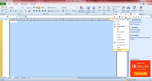
You can hide columns from the Excel spreadsheets much the same. Select a few of the column headings to remove from the spreadsheets whilst pressing Ctrl. Note that they don’t necessarily have to be adjacent columns. Right-click one of the selected column headings, and then click Hide to remove them as in the shot below.

Then select the columns to the left and right of the ones that are hidden from view. Then you should right-click on the selected column headings, and select Unhide from the context menu. The hidden columns will then reappear in the Excel spreadsheet.

Hiding columns and rows might be handy for shrinking larger Excel 2010/13 spreadsheets down to size. In addition, with the Hide/Unhide options you can also print the most relevant columns and rows from spreadsheets without having to delete anything from them.