Excel 2010/2013 doesn’t have any specific options that add watermarks to spreadsheets. However, you can still add watermark images and text to spreadsheets. Add the watermarks to the spreadsheets with Excel’s header and footer tools.

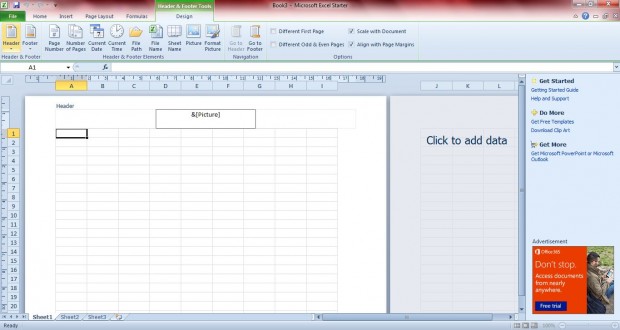
Open an Excel spreadsheet, and click the Insert tab. Then select the Header and Footer option to add a header as below. Then you should select the middle of the header.

Then click the Picture option, choose a suitable watermark image and select Insert. As you still have the header open the picture is not displayed, but the header still includes &[Picture]. Insert blank lines before &[Picture] center the image within the header.

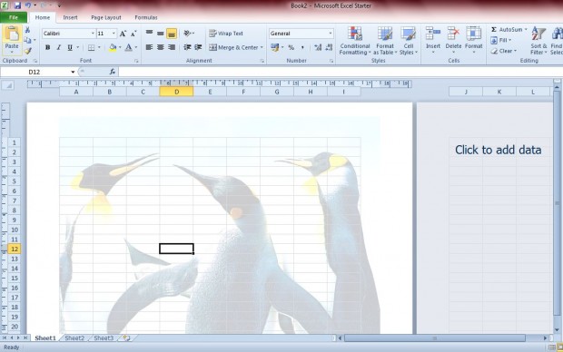
To view the picture, you should click on a cell outside of the header. Then the image is displayed, full-color, behind the spreadsheet cells as in the shot below. As such, you must still fade the image to remove its colors.

Click on the header again, and select the Format Picture option from Header and Footer Tools tab. That opens the window below where you should select the Picture tab. Select Washout from the Color drop-down list, and click OK to close the window.  Now you should find that the watermark image you added is faded behind the spreadsheet cells.

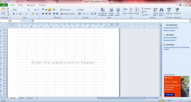
Thus, the spreadsheet now has a watermark image. You can also add text watermarks to the spreadsheets by replacing the & [Picture] in the header with some alternative text. Then select and format the text, and click the Font Color option. From the palette, choose a faded, light grey font color for the text.

Place the cursor just in front of the header text, and press Return to move it further down the spreadsheet page so that’s in the middle of the page. Then click a cell outside of the header, and the text becomes a spreadsheet watermark as below. However, you cannot change the text direction of the watermark.

Now you can add both image and text watermarks to your spreadsheet documents. Add the watermarks to indicate a spreadsheet document status, or include a logo image in the background.