A pictograph is a graph with pictures. The number of pictures in the graph shows you a specific value. Excel 2010 does not include any direct options to set up pictographs, but with a little customization you can convert bar graphs to pictographs.

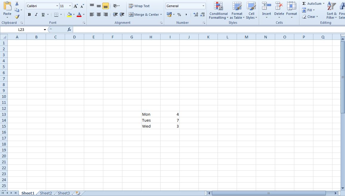
Open Excel and enter the values for your graph. For a bar graph you should enter a couple of columns into the sheets as shown below. The columns will be the X and Y axis.

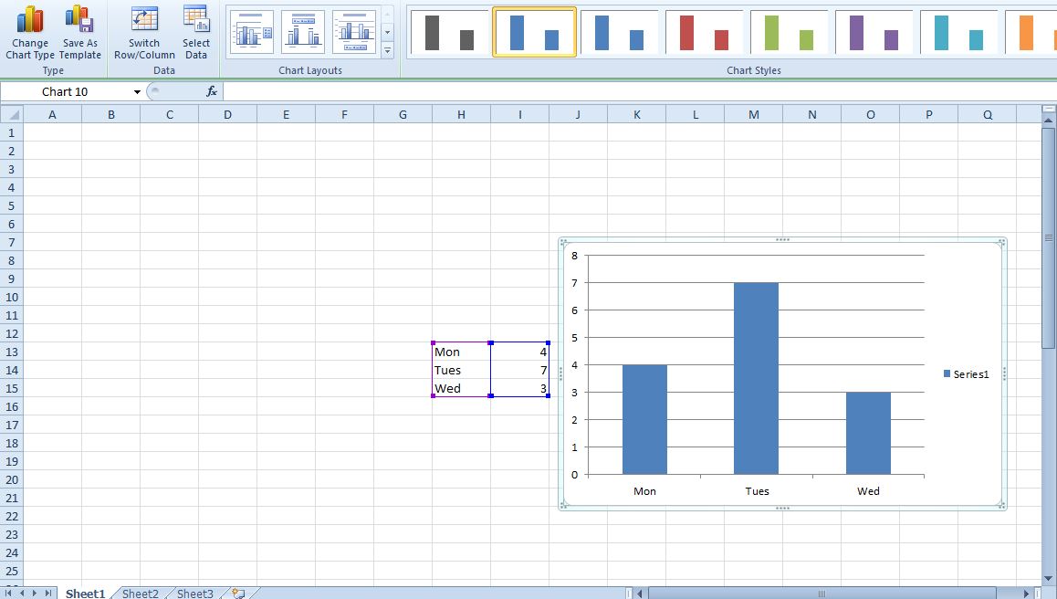
Next, select the cells within the two columns and click the Insert tab. Press the Column button, and select one of the 2D column charts. That will add a column, or bar, graph to the spreadsheet as shown in the shot below.

Now click the Clip Art button on the Insert tab. That will open Excel’s clip art as shown below. Enter a keyword in the search box to find a clip art image to add to the graph.

Right-click on the selected clip art and select Copy. Then click on one of the bars on the chart to select them. Press Ctrl + V to paste the picture into the bars as below.

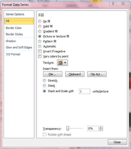
Now right-click on the bars and select Format Data Series to open the window below. Click Fill on that window, and then select the Stack and Scale with option. Do not enter any number in the adjacent text box, and press the Close button.

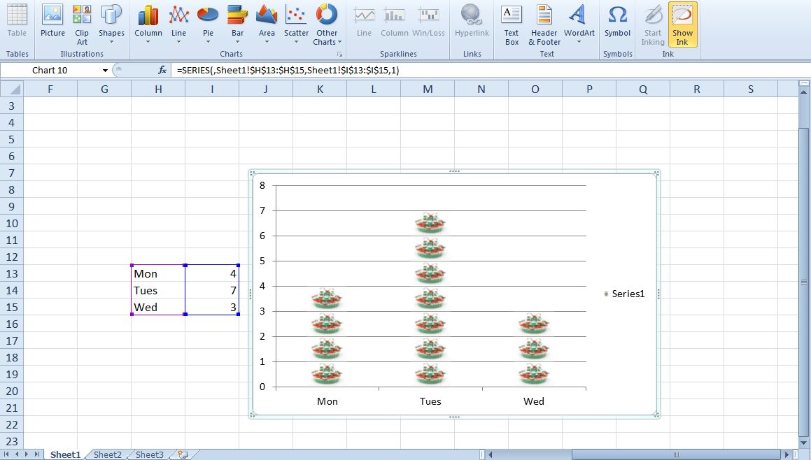
Then you’ll have a pictograph as in the shot below. Thus, the bars are now replaced with images. The number of images in each column is the same as the value entered in the graph’s spreadsheet cells.

A pictograph option is something Microsoft should have already incorporated in Excel. Nevertheless, for now you can set up some great pictographs by converting the bar graphs.