Excel’s PMT function is one that calculates the monthly payments required to clear a loan over a specific period. So if you’ve taken a loan out, you can find out exactly what you need to pay each month to clear it over a certain period. The function assumes that the loan has a fixed interest rate. 

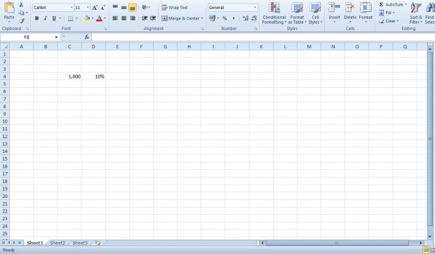
For example, let’s suppose you have a 1,000 loan with a 10% APR fixed interest rate and need to clear it in 24 months. First, enter 1,000 in an Excel spreadsheet cell. Enter the 10% interest rate in an adjacent cell as shown in the shot below.

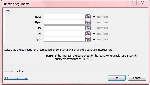
Now select a third cell to add the function to, and press the fx button. Then select the PMT function. That opens the window in the shot below.

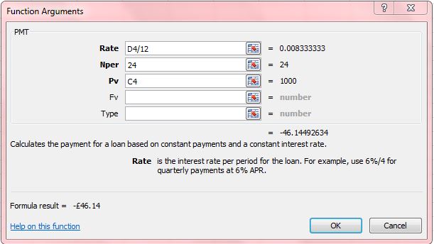
First, press the button beside the Rate text box to select the cell with the interest rate in. In addition, add /12 after the cell reference. So it should be something like D4/12, which will highlight the loan is cleared monthly. If it were on a quarterly basis you would enter /4.

Next, enter the time period for the loan in the Nper text box. Note that is entered in months. So a couple of years would be 24 months. Alternatively, you could also enter it as 2*12.

Then press the button beside the Pv text box and select the cell with the loan total in it. Leave the Fv and Type boxes blank. The PMT window should match the one in the shot below.

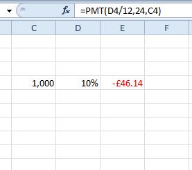
Press the OK button to close the window. The PMT function cell will now show you the monthly payment required to clear the loan in exactly 24 months as in the shot below. When multiplied by 24, that cell amounts to a total value of 1,107.36.

So with this function you can now quickly find out the exact instalments required to clear a loan in certain time frame. For further details, check out this YouTube page that includes an Excel PMT video.