The plot area of an Excel spreadsheet graph is the inner border and background area of the chart. Excel 2010/2013 includes a variety of options to customize the plot area with. For example, you can add glow effects, shadows and a 3D format to the plot area border.

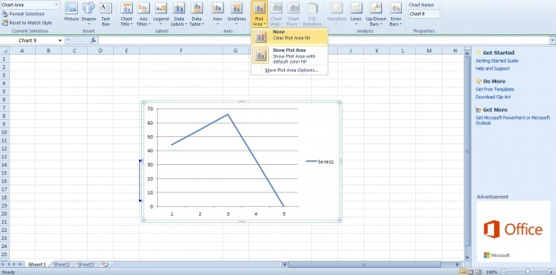
First, enter the numbers for your graph in an Excel spreadsheet. Select those numbers, click Insert and then choose a graph to add to the document as below. Click Layout and select Plot Area to open a submenu with a couple of options on it.

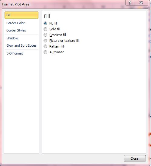
There you can select None to remove the plot area from the chart if it’s not required. If you’re going to keep the plot area on the chart, select More Plot Area Options. That will open the window in the snapshot below.

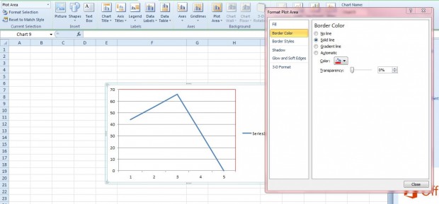
Firstly, you can choose alternative colors for the border. Click Border Color and Solid line, and then select Color to open the palette. From there you can choose a color for the plot area border.

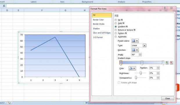
To add alternative colors to the plot area background, click Fill on the formatting window. Then select either Solid fill or Gradient fill. If you select Gradient fill, as below, you can choose a variety of gradients with the Presets colors option. Select the Direction option to choose alternative directions for the gradients.

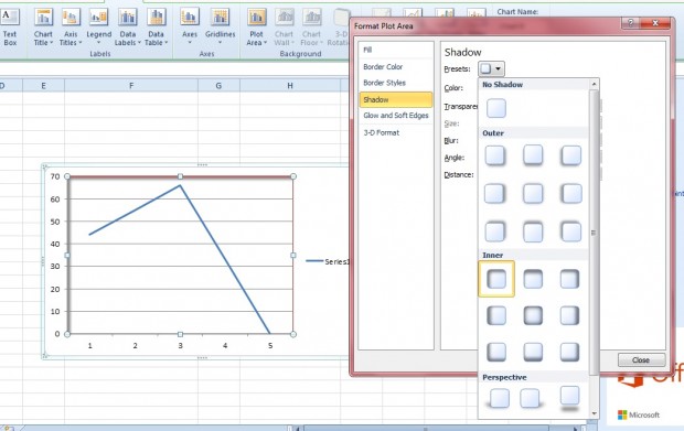
Add shadows to the plot area by selecting Shadow. Then select Presets to open shadow options as shown in the shot below. There you can add shadows to the graph’s inner or outer plot areas.

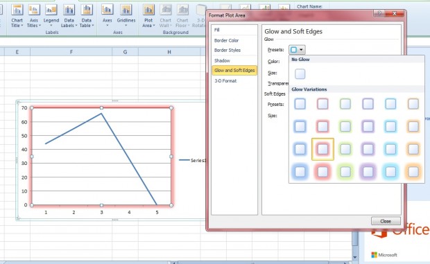
Below Shadow you can select Glow and Soft Edges. Click Presets to choose a glow variation. Drag the Size and Transparency bars to further customize the glow effect.

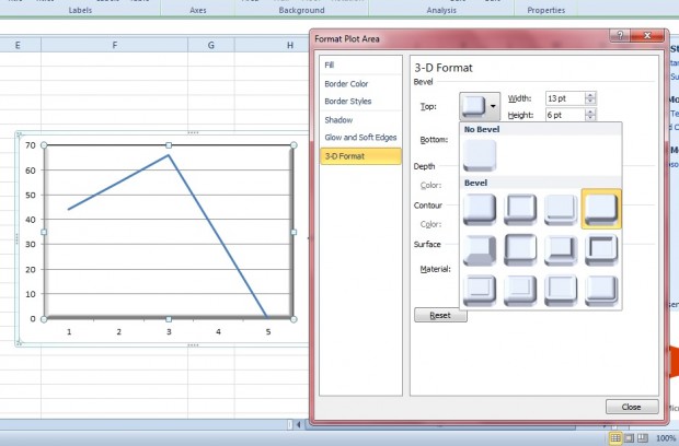
You can also add 3D format effects to the graphs by selecting 3-D Format option. Then you can add 3D effects to the plot area by clicking the Top or Bottom options. That opens a menu with various Bevel effect options on it.

Those are a few of the options you can format plot areas in Excel graphs with. They’ll add a little more pizzazz to your spreadsheet charts.