If you have opened a large OpenOffice spreadsheet document, it might be handy to keep some of its rows and columns stationary. OpenOffice Calc has an option with which you can freeze selected columns and rows so that they always remain visible, even if you have scrolled some way down or across the spreadsheet. As such, with the freeze option you can lock a number of rows and columns on the top or left of a spreadsheet.

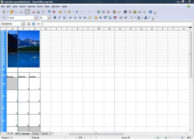
Open a OpenOffice spreadsheet, and then click on a column header to the right of where you want to freeze. Then you should click Window and the Freeze option from the menu. A dark line should appear on the spreadsheet, as in the shot below, which highlights where you placed the freeze. Now move the scroll bar to the right, and the frozen column remain stationary on the left of the spreadsheet.

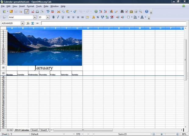
To freeze spreadsheet rows, click on the header of the row (its number) directly below where you intend to freeze it. Click on Window and the Freeze option to add a dark line that runs across the spreadsheet as below. All the rows above that line are frozen, and they will stay at the top of the spreadsheet when you scroll down the page.

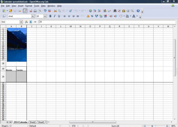
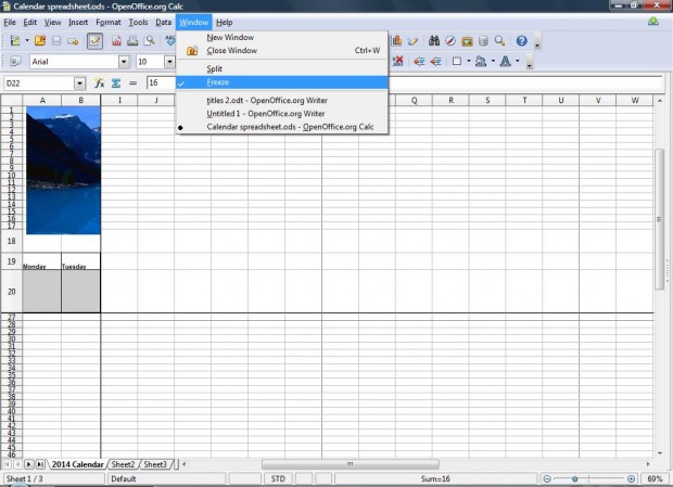
You can also freeze both rows and columns. Click on a cell that is immediately below the row and just to the right of columns that you’re going to freeze. Select Window > Freeze and both a horizontal and vertical line will then appear on your spreadsheet as below. All the rows above and columns to the left of those lines remain in view as you scroll across the spreadsheet.

Having frozen the rows and columns, you can also unfreeze them. Click Window > Freeze to remove the checkmark beside the option. That removes the horizontal/vertical freeze lines that were on the spreadsheet.

You can also freeze rows and columns much the same with alternative spreadsheet packages such as Excel. This is a handy option for keeping row and column labels visible in spreadsheets.