In Google Sheets, there are formatting options that lets you format any numerical data on certain rows, columns or cells to currency, percentage, decimals, etc. Now, what if the format that you want isn’t available in the given options? Is there a way for you to create your own number format? Well, there is and that’s what you are about to learn in this post.

How to use custom number format in Google Sheets

• Create a new blank spreadsheet in Google Sheets.
• On your blank spreadsheet, fill in the cells, rows or columns with the numerical data that you want.
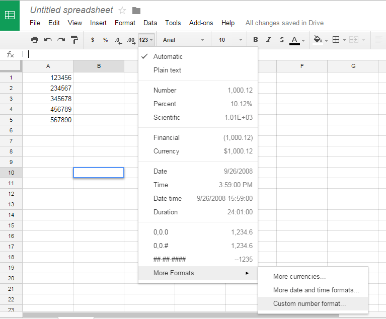
• After doing so, click the “More formats” icon in the toolbar (see image below).

• Under the More formats menu, select “More formats” > “Custom number format”.

• On the custom number format field, enter the type of format that you want. You can also select from the available formats on the list.

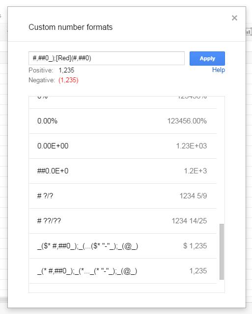
• To set up your own format, you need to keep in mind that a custom format can be composed of up to four parts: positive, negative, zero and text. Each part must be separated by a semicolon.
• You should also keep in mind that you can only use the supported characters. You can also use colors to distinguish certain values or numbers (ex. positive numbers and negative numbers).
• So after setting up your custom number format, click the “Apply” button to confirm.
• Next, apply the custom number formatting to any cell, column or row in your spreadsheet. Make sure to highlight your data first and then click the “More formats” icon again. Select your custom number format on the menu.

So that’s it. You’re done. If you wish to learn more about custom number formatting in Google Sheets, you can refer to this article.